Nous poursuivons notre introduction à matplotlib avec les visualisations en 3 dimensions. Comme pour la première partie sur les fonctions en 2 dimensions, nous allons seulement paraphraser le tutoriel en ligne, avec l’avantage toutefois que nous procurent les notebooks.
# la ration habituelle d'imports
import matplotlib.pyplot as plt
# et aussi numpy, même si ça n'est pas strictement nécessaire
import numpy as np
Pour pouvoir faire des visualisations en 3D, il vous faut importer ceci :
# même si l'on n'utilise pas explicitement
# d'attributs du module Axes3D
# cet import est nécessaire pour faire
# des visualisations en 3D
from mpl_toolkits.mplot3d import Axes3D
Dans ce notebook nous allons utiliser un mode de visualisation un peu plus élaboré, mieux intégré à l’environnement des notebooks :
# ce mode d'interaction va nous permettre de nous déplacer
# dans l'espace pour voir les courbes en 3D
# depuis plusieurs points de vue
%matplotlib ipympl
Comme on va le voir très vite, avec ces réglages vous aurez la possibilité d’explorer interactivement les visualisations en 3D.
Un premier exemple : une courbe
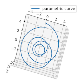
Commençons par le premier exemple du tutorial, qui nous montre comment dessiner une ligne suivant une courbe définie de manière paramétrique (ici, et sont fonctions de ). Les points importants sont :
la composition d’un plot (plusieurs figures, chacune composée de plusieurs subplots), reste bien entendu valide ; j’ai enrichi l’exemple initial pour mélanger un subplot en 3D avec un subplot en 2D ;
l’utilisation du paramètre
projection='3d'lorsqu’on crée un subplot qui va se prêter à une visualisation en 3D ;l’objet subplot ainsi créé est une instance de la classe
Axes3DSubplot;on peut envoyer à cet objet :
la méthode
plotqu’on avait déjà vue pour la dimension 2 (c’est ce que l’on fait dans ce premier exemple) ;des méthodes spécifiques à la 3D, que l’on voit dans les exemples suivants.
# je choisis une taille raisonnable compte tenu de l'espace
# disponible dans fun-mooc
fig = plt.figure(figsize=(6, 3))

# voici la façon de créer un *subplot*
# qui se prête à une visualisation en 3D
ax = fig.add_subplot(121, projection='3d')

# à présent, copié de
# https://matplotlib.org/mpl_toolkits/mplot3d/tutorial.html#line-plots
# on crée une courbe paramétrique
# où x et y sont fonctions de z
theta = np.linspace(-4 * np.pi, 4 * np.pi, 100)
z = np.linspace(-2, 2, 100)
r = z**2 + 1
x = r * np.sin(theta)
y = r * np.cos(theta)
# on fait maitenant un appel à plot normal
# mais avec un troisième paramètre
ax.plot(x, y, z, label='parametric curve')
ax.legend()

# on peut tout à fait ajouter un plot usuel
# dans un subplot, comme on l'a vu pour la 2D
ax2 = fig.add_subplot(122)
x = np.linspace(0, 10)
y = x**2
ax2.plot(x, y)
plt.show()Un autre point à remarquer est qu’avec le mode d’interaction que nous avons choisi :
%matplotlib ipymplvous bénéficiez d’un mode d’interaction plus riche avec la figure (nb: ça nécessite l’installation de pip install ipympl). Par exemple, vous pouvez cliquer dans la figure en 3D, et vous déplacer pour changer de point de vue ; par exemple si vous sélectionnez l’outil Pan/Zoom (l’outil avec 4 flèches), vous pouvez arriver à voir ceci :
Les différents boutons d’outil sont décrits plus en détail ici. Je dois avouer ne pas arriver à tout utiliser lorsque la visualisation est faite dans un notebook, mais la possibilité de modifier le point de vue peut s’avérer intéressante pour explorer les données.
En explorant les autres exemples du tutorial, vous pouvez commencer à découvrir l’éventail des possibilités offertes par matplotlib.
Axes3DSubplot.scatter
Comme en dimension 2, scatter permet de montrer un nuage de points.
Tutoriel original : https://
scatter3d_demo.py
'''
==============
3D scatterplot
==============

Demonstration of a basic scatterplot in 3D.
'''

from mpl_toolkits.mplot3d import Axes3D
import matplotlib.pyplot as plt
import numpy as np
The history saving thread hit an unexpected error (OperationalError('database is locked')).History will not be written to the database.
fig = plt.figure(figsize=(4, 4))

def randrange(n, vmin, vmax):
    '''
    Helper function to make an array of random numbers having shape (n, )
    with each number distributed Uniform(vmin, vmax).
    '''
    return (vmax - vmin)*np.random.rand(n) + vmin

ax = fig.add_subplot(111, projection='3d')

n = 100

# For each set of style and range settings, plot n random points in the box
# defined by x in [23, 32], y in [0, 100], z in [zlow, zhigh].
for c, m, zlow, zhigh in [('r', 'o', -50, -25), ('b', '^', -30, -5)]:
    xs = randrange(n, 23, 32)
    ys = randrange(n, 0, 100)
    zs = randrange(n, zlow, zhigh)
    ax.scatter(xs, ys, zs, c=c, marker=m)

ax.set_xlabel('X Label')
plt.show()Axes3DSubplot.plot_wireframe
Utilisez cette méthode pour dessiner en mode “fil de fer”.
Tutoriel original : https://
wire3d_demo.py
from mpl_toolkits.mplot3d import axes3dfig = plt.figure(figsize=(4, 4))
ax = fig.add_subplot(111, projection='3d')
# Grab some test data.
X, Y, Z = axes3d.get_test_data(0.05)
# Plot a basic wireframe.
ax.plot_wireframe(X, Y, Z, rstride=10, cstride=10)
plt.show()Axes3DSubplot.plot_surface
Comme on s’en doute, plot_surface sert à dessiner des surfaces dans l’espace ; ces exemples montrent surtout comment utiliser des couleurs ou des patterns.
Tutoriel original : https://
surface3d_demo.py
'''
======================
3D surface (color map)
======================

Demonstrates plotting a 3D surface colored with the coolwarm color map.
The surface is made opaque by using antialiased=False.

Also demonstrates using the LinearLocator and custom formatting for the
z axis tick labels.
'''

from mpl_toolkits.mplot3d import Axes3D
import matplotlib.pyplot as plt
from matplotlib import cm
from matplotlib.ticker import LinearLocator, FormatStrFormatter
import numpy as np
fig = plt.figure(figsize=(4, 4))
# dans le tuto on trouve
# fig, ax = plt.subplots(subplot_kw=dict(projection='3d'))
# personnellement je trouve plus facile à retenir ceci
ax = fig.add_subplot(111, projection='3d')
# Make data.
X = np.arange(-5, 5, 0.25)
Y = np.arange(-5, 5, 0.25)
X, Y = np.meshgrid(X, Y)
R = np.sqrt(X**2 + Y**2)
Z = np.sin(R)
# Plot the surface.
surf = ax.plot_surface(X, Y, Z, cmap=cm.coolwarm,
linewidth=0, antialiased=False)
# Customize the z axis.
ax.set_zlim(-1.01, 1.01)
ax.zaxis.set_major_locator(LinearLocator(10))
ax.zaxis.set_major_formatter(FormatStrFormatter('%.02f'))
# Add a color bar which maps values to colors.
fig.colorbar(surf, shrink=0.5, aspect=5)
plt.show()surface3d_demo2.py
'''
========================
3D surface (solid color)
========================

Demonstrates a very basic plot of a 3D surface using a solid color.
'''

from mpl_toolkits.mplot3d import Axes3D
import matplotlib.pyplot as plt
import numpy as np
fig = plt.figure(figsize=(4, 4))
ax = fig.add_subplot(111, projection='3d')
# Make data
u = np.linspace(0, 2 * np.pi, 30)
v = np.linspace(0, np.pi, 30)
x = 10 * np.outer(np.cos(u), np.sin(v))
y = 10 * np.outer(np.sin(u), np.sin(v))
z = 10 * np.outer(np.ones(np.size(u)), np.cos(v))
# Plot the surface
ax.plot_surface(x, y, z, color='b')
plt.show()surface3d_demo3.py
'''
=========================
3D surface (checkerboard)
=========================

Demonstrates plotting a 3D surface colored in a checkerboard pattern.
'''

from mpl_toolkits.mplot3d import Axes3D
import matplotlib.pyplot as plt
from matplotlib import cm
from matplotlib.ticker import LinearLocator
import numpy as np
fig = plt.figure(figsize=(4, 4))
ax = fig.add_subplot(111, projection='3d')
# Make data.
X = np.arange(-5, 5, 0.25)
xlen = len(X)
Y = np.arange(-5, 5, 0.25)
ylen = len(Y)
X, Y = np.meshgrid(X, Y)
R = np.sqrt(X**2 + Y**2)
Z = np.sin(R)
# Create an empty array of strings with the same shape as the meshgrid, and
# populate it with two colors in a checkerboard pattern.
colortuple = ('y', 'b')
colors = np.empty(X.shape, dtype=str)
for y in range(ylen):
for x in range(xlen):
colors[x, y] = colortuple[(x + y) % len(colortuple)]
# Plot the surface with face colors taken from the array we made.
surf = ax.plot_surface(X, Y, Z, facecolors=colors, linewidth=0)
# Customize the z axis.
ax.set_zlim(-1, 1)
# 2023 Dec: this line breaks the script, although it's still
# in matplotlib's examples; let's ignore it for now
# ax.w_zaxis.set_major_locator(LinearLocator(6))
plt.show()Axes3DSubplot.plot_trisurf
plot_trisurf se prête aussi au rendu de surfaces, mais sur la base de maillages en triangles.
Tutoriel original : https://
trisurf3d_demo.py
'''
======================
Triangular 3D surfaces
======================

Plot a 3D surface with a triangular mesh.
'''

from mpl_toolkits.mplot3d import Axes3D
import matplotlib.pyplot as plt
import numpy as np
fig = plt.figure(figsize=(4, 4))
ax = fig.add_subplot(111, projection='3d')
n_radii = 8
n_angles = 36
# Make radii and angles spaces (radius r=0 omitted to eliminate duplication).
radii = np.linspace(0.125, 1.0, n_radii)
angles = np.linspace(0, 2*np.pi, n_angles, endpoint=False)
# Repeat all angles for each radius.
angles = np.repeat(angles[..., np.newaxis], n_radii, axis=1)
# Convert polar (radii, angles) coords to cartesian (x, y) coords.
# (0, 0) is manually added at this stage, so there will be no duplicate
# points in the (x, y) plane.
x = np.append(0, (radii*np.cos(angles)).flatten())
y = np.append(0, (radii*np.sin(angles)).flatten())
# Compute z to make the pringle surface.
z = np.sin(-x*y)
ax.plot_trisurf(x, y, z, linewidth=0.2, antialiased=True)
plt.show()trisurf3d_demo2.py
'''
===========================
More triangular 3D surfaces
===========================

Two additional examples of plotting surfaces with triangular mesh.

The first demonstrates use of plot_trisurf's triangles argument, and the
second sets a Triangulation object's mask and passes the object directly
to plot_trisurf.
'''

import numpy as np
import matplotlib.pyplot as plt
from mpl_toolkits.mplot3d import Axes3D
import matplotlib.tri as mtri
fig = plt.figure(figsize=(6, 3))
#============
# First plot
#============
# Make a mesh in the space of parameterisation variables u and v
u = np.linspace(0, 2.0 * np.pi, endpoint=True, num=50)
v = np.linspace(-0.5, 0.5, endpoint=True, num=10)
u, v = np.meshgrid(u, v)
u, v = u.flatten(), v.flatten()
# This is the Mobius mapping, taking a u, v pair and returning an x, y, z
# triple
x = (1 + 0.5 * v * np.cos(u / 2.0)) * np.cos(u)
y = (1 + 0.5 * v * np.cos(u / 2.0)) * np.sin(u)
z = 0.5 * v * np.sin(u / 2.0)
# Triangulate parameter space to determine the triangles
tri = mtri.Triangulation(u, v)
# Plot the surface. The triangles in parameter space determine which x, y, z
# points are connected by an edge.
ax = fig.add_subplot(1, 2, 1, projection='3d')
ax.plot_trisurf(x, y, z, triangles=tri.triangles, cmap=plt.cm.Spectral)
ax.set_zlim(-1, 1)
#============
# Second plot
#============
# Make parameter spaces radii and angles.
n_angles = 36
n_radii = 8
min_radius = 0.25
radii = np.linspace(min_radius, 0.95, n_radii)
angles = np.linspace(0, 2*np.pi, n_angles, endpoint=False)
angles = np.repeat(angles[..., np.newaxis], n_radii, axis=1)
angles[:, 1::2] += np.pi/n_angles
# Map radius, angle pairs to x, y, z points.
x = (radii*np.cos(angles)).flatten()
y = (radii*np.sin(angles)).flatten()
z = (np.cos(radii)*np.cos(angles*3.0)).flatten()
# Create the Triangulation; no triangles so Delaunay triangulation created.
triang = mtri.Triangulation(x, y)
# Mask off unwanted triangles.
xmid = x[triang.triangles].mean(axis=1)
ymid = y[triang.triangles].mean(axis=1)
mask = np.where(xmid**2 + ymid**2 < min_radius**2, 1, 0)
triang.set_mask(mask)
# Plot the surface.
ax = fig.add_subplot(1, 2, 2, projection='3d')
ax.plot_trisurf(triang, z, cmap=plt.cm.CMRmap)
plt.show()Axes3DSubplot.contour
Pour dessiner des contours.
Tutoriel original : https://
contour3d_demo.py
from mpl_toolkits.mplot3d import axes3d
import matplotlib.pyplot as plt
from matplotlib import cm
fig = plt.figure(figsize=(4, 4))
ax = fig.add_subplot(111, projection='3d')
X, Y, Z = axes3d.get_test_data(0.05)
cset = ax.contour(X, Y, Z, cmap=cm.coolwarm)
ax.clabel(cset, fontsize=9, inline=1)
plt.show()contour3d_demo2.py
from mpl_toolkits.mplot3d import axes3d
import matplotlib.pyplot as plt
from matplotlib import cm
fig = plt.figure(figsize=(4, 4))
ax = fig.add_subplot(111, projection='3d')
X, Y, Z = axes3d.get_test_data(0.05)
cset = ax.contour(X, Y, Z, extend3d=True, cmap=cm.coolwarm)
ax.clabel(cset, fontsize=9, inline=1)
plt.show()contour3d_demo3.py
from mpl_toolkits.mplot3d import axes3d
import matplotlib.pyplot as plt
from matplotlib import cm
fig = plt.figure(figsize=(4, 4))
ax = fig.add_subplot(111, projection='3d')
X, Y, Z = axes3d.get_test_data(0.05)
ax.plot_surface(X, Y, Z, rstride=8, cstride=8, alpha=0.3)
cset = ax.contour(X, Y, Z, zdir='z', offset=-100, cmap=cm.coolwarm)
cset = ax.contour(X, Y, Z, zdir='x', offset=-40, cmap=cm.coolwarm)
cset = ax.contour(X, Y, Z, zdir='y', offset=40, cmap=cm.coolwarm)
ax.set_xlabel('X')
ax.set_xlim(-40, 40)
ax.set_ylabel('Y')
ax.set_ylim(-40, 40)
ax.set_zlabel('Z')
ax.set_zlim(-100, 100)
plt.show()Axes3DSubplot.contourf
Comme Axes3DSubplot.contour, mais avec un rendu plein plutôt que sous forme de lignes (le f provient de l’anglais filled).
Tutoriel original : https://
contourf3d_demo.py
from mpl_toolkits.mplot3d import axes3d
import matplotlib.pyplot as plt
from matplotlib import cm
fig = plt.figure(figsize=(4, 4))
ax = fig.add_subplot(111, projection='3d')
X, Y, Z = axes3d.get_test_data(0.05)
cset = ax.contourf(X, Y, Z, cmap=cm.coolwarm)
ax.clabel(cset, fontsize=9, inline=1)
plt.show()contourf3d_demo2.py
"""
.. versionadded:: 1.1.0
   This demo depends on new features added to contourf3d.
"""

from mpl_toolkits.mplot3d import axes3d
import matplotlib.pyplot as plt
from matplotlib import cm
fig = plt.figure(figsize=(4, 4))
ax = fig.add_subplot(111, projection='3d')
X, Y, Z = axes3d.get_test_data(0.05)
ax.plot_surface(X, Y, Z, rstride=8, cstride=8, alpha=0.3)
cset = ax.contourf(X, Y, Z, zdir='z', offset=-100, cmap=cm.coolwarm)
cset = ax.contourf(X, Y, Z, zdir='x', offset=-40, cmap=cm.coolwarm)
cset = ax.contourf(X, Y, Z, zdir='y', offset=40, cmap=cm.coolwarm)
ax.set_xlabel('X')
ax.set_xlim(-40, 40)
ax.set_ylabel('Y')
ax.set_ylim(-40, 40)
ax.set_zlabel('Z')
ax.set_zlim(-100, 100)
plt.show()Axes3DSubplot.add_collection3d
Pour afficher des polygones.
Tutoriel original : https://
"""
=============================================
Generate polygons to fill under 3D line graph
=============================================

Demonstrate how to create polygons which fill the space under a line
graph. In this example polygons are semi-transparent, creating a sort
of 'jagged stained glass' effect.
"""

from mpl_toolkits.mplot3d import Axes3D
from matplotlib.collections import PolyCollection
import matplotlib.pyplot as plt
from matplotlib import colors as mcolors
import numpy as np
fig = plt.figure(figsize=(4, 4))
ax = fig.add_subplot(111, projection='3d')
def cc(arg):
return mcolors.to_rgba(arg, alpha=0.6)
xs = np.arange(0, 10, 0.4)
verts = []
zs = [0.0, 1.0, 2.0, 3.0]
for z in zs:
ys = np.random.rand(len(xs))
ys[0], ys[-1] = 0, 0
verts.append(list(zip(xs, ys)))
poly = PolyCollection(verts, facecolors=[cc('r'), cc('g'), cc('b'),
cc('y')])
poly.set_alpha(0.7)
ax.add_collection3d(poly, zs=zs, zdir='y')
ax.set_xlabel('X')
ax.set_xlim3d(0, 10)
ax.set_ylabel('Y')
ax.set_ylim3d(-1, 4)
ax.set_zlabel('Z')
ax.set_zlim3d(0, 1)
plt.show()Axes3DSubplot.bar
Pour construire des diagrammes à barres.
Tutoriel original : https://
bars3d_demo.py
"""
========================================
Create 2D bar graphs in different planes
========================================

Demonstrates making a 3D plot which has 2D bar graphs projected onto
planes y=0, y=1, etc.
"""

from mpl_toolkits.mplot3d import Axes3D
import matplotlib.pyplot as plt
import numpy as np
fig = plt.figure(figsize=(4, 4))
ax = fig.add_subplot(111, projection='3d')
for c, z in zip(['r', 'g', 'b', 'y'], [30, 20, 10, 0]):
xs = np.arange(20)
ys = np.random.rand(20)
# You can provide either a single color or an array. To demonstrate this,
# the first bar of each set will be colored cyan.
cs = [c] * len(xs)
cs[0] = 'c'
ax.bar(xs, ys, zs=z, zdir='y', color=cs, alpha=0.8)
ax.set_xlabel('X')
ax.set_ylabel('Y')
ax.set_zlabel('Z')
plt.show()Axes3DSubplot.quiver
Pour afficher des champs de vecteurs sous forme de traits.
Tutoriel original : https://
quiver3d_demo.py
'''
==============
3D quiver plot
==============

Demonstrates plotting directional arrows at points on a 3d meshgrid.
'''

from mpl_toolkits.mplot3d import axes3d
import matplotlib.pyplot as plt
import numpy as np
fig = plt.figure(figsize=(4, 4))
ax = fig.add_subplot(111, projection='3d')
# Make the grid
x, y, z = np.meshgrid(np.arange(-0.8, 1, 0.2),
np.arange(-0.8, 1, 0.2),
np.arange(-0.8, 1, 0.8))
# Make the direction data for the arrows
u = np.sin(np.pi * x) * np.cos(np.pi * y) * np.cos(np.pi * z)
v = -np.cos(np.pi * x) * np.sin(np.pi * y) * np.cos(np.pi * z)
w = (np.sqrt(2.0 / 3.0) * np.cos(np.pi * x) * np.cos(np.pi * y) *
np.sin(np.pi * z))
ax.quiver(x, y, z, u, v, w, length=0.1, normalize=True)
plt.show()